Generating Correlated Data from Linear Models

The standard linear regression model is as follows:

	y = b0 + b1*x + e

There are three parameters in this model. First, b0 is the y-intercept: the expected value of y when x = 0. b1 is the weight for x: the expected change in y for a one- unit change in x. The third parameter, which isn't noted explicitly, is the variance of the residual term. (The residuals are assumed to be normally distributed with a mean of 0. But the variance of the residuals is a parameter to be specified in simulations or estimated in empirical analyses.)

Thus, we can generate data that follow a given regression model by plugging in different values for the three parameters. In the example below I have used a value of 10 for b0, .50 for b1, and .1 for the resid SD.

	n = 1000
	x = rnorm(n)
	y = 10 + .5*x + rnorm(n,0,.1)
	plot(x,y); summary(lm(y~x)); cor(x,y)

We can adjust the residual variance by changing the SD of the normal distribution from which the residuals are being sampled:

	x = rnorm(n)
	y = 10 + .5*x + rnorm(n,0,2)
	plot(x,y); summary(lm(y~x)); cor(x,y)

Important: Notice that the estimate of b1 is not equivalent to r. When we specify the value of b1, we are simply noting how much the expected value of y should change with a 1 unit increase in x. But there is variation around that expected value. That variation is controlled by the residual variance. The larger the resid variance, the more scatter there is around the expected line. The more scatter there is, the weaker the correlation will be even when b1 is constant. You can see this by exploring different values of residual variance while constraining b1 to .50, as we did above.

If we want to manipulate the correlation per se, it is helpful to keep in mind that the correlation is equivalent to the regression weight for a regression model based on standardized scores. In such a situation, y has a variance or SD of 1.00. If x accounts for 50% of the variance in y, then the residual must account for the remaining variance (1 - 50%) = 50%. The SD (sqrt of the var) for the error term must reflect this if the goal of the simulation is to vary the correlation itself.

	b1 = .50
	x = rnorm(n)
	y = 10 + b1*x + rnorm(n,0,sqrt(1-b1^2))
	plot(x,y); summary(lm(y~x)); cor(x,y)
	

In the example above, we have created a situation in which x (which has a SD of approximately 1) accounts for b1^2 of the variance in y. Thus, the residual accounts for 1 - b1^2 of the variance. This allows y to be standardized (var = 1) and allows the regression weight to be comparable to the correlation.

Multiple Regression

Generating data using multiple predictors is a bit more complex and requires using libraries or your knowledge of psychometrics, SEM, etc. If two predictors are independent, then we can use the same logic described above to model y. Namely, the residual will have a variance equivalent to the VAR(y) - the variance explained by x1 and x2:

	b1 = .10
	b2 = .20
	x1 = rnorm(n)
	x2 = rnorm(n)
	y = 10 + b1*x1 + b2*x2 + rnorm(n,0,sqrt(1 - ((b1^2) + (b2^2)) ))
	summary(lm(y ~ x1 + x2)); cor(x1,x2); cor(x1,y); cor(x2,y)

If the predictors are correlated (not independent), then there is an overlapping portion of variance that each predictor is contributing to y. This will inflate the variance of y in undesirable ways if it is not weighted appropriately. This can be seen in the following example. Notice that the var of Y is a tiny bit larger than it should be (1.00).

	r = .9
	x1 = rnorm(n)
	x2 = r*x1 + rnorm(n,0,sqrt(1-r^2))
	cor(x1,x2)
	y = 10 + b1*x1 + b2*x2 + rnorm(n,0,sqrt(1 - ((b1^2) + (b2^2)) ) )

	summary(lm(y ~ x1 + x2)) 
	cor(x1,x2); cor(x1,y); cor(x2,y)
	sd(x1); sd(x2); sd(y); var(y)

The variance of a composite (y) is equal to the weighted sum of the var-cov matrix of components (predictors): (b1^2) + (b2^2) + (2*b1*b2*r). Thus, in our example, the var of y is inflated by (2*b1*b2*r). That isn't much in this simple example (about .036), but there are situations where we wouldn't want this error to compound itself. We can correct for by adjusting the variance of the residual term accordingly):

	r = .9
	x1 = rnorm(n)
	x2 = r*x1 + rnorm(n,0,sqrt(1-r^2))
	cor(x1,x2)
	y = 10 + b1*x1 + b2*x2 + rnorm(n,0,sqrt(1 - ((b1^2) + (b2^2) + (2*b1*b2*r))))

	summary(lm(y ~ x1 + x2))
	cor(x1,y); cor(x2,y)
	sd(x1); sd(x2); sd(y)

If one has some familiarity with matrix algebra and SEM, one can generate a variety of complex multivariate structures. We will elaborate on such ideas in later sessions. To give you a flavor for this process, however, I'll present a final example in which we assume a latent factor leads to correlated scores on 4 different measures/variables/tests:

	latent.factor = rnorm(n)
	loading = .707
	x1 = loading*latent.factor + rnorm(n,0,sqrt(1-loading^2))
	x2 = loading*latent.factor + rnorm(n,0,sqrt(1-loading^2))
	x3 = loading*latent.factor + rnorm(n,0,sqrt(1-loading^2))
	x4 = loading*latent.factor + rnorm(n,0,sqrt(1-loading^2))

	x = cbind(x1,x2,x3,x4)	# let's collect the four variables into a matrix
	x = data.frame(x)	# place them into a data frame
	cor(x)			# correlation matrix for measurements

The average correlation among these measures should be .50. In later examples, we will use factor analysis to estimate the loadings for a common factor model and see if we can recover the true loadings (.707).

lavaan

An R Library for Latent Variable Modeling (LVM) and Analysis

One of the fun things about R is that developers can create packages or libraries that users can download to perform specialized tasks in R. There are, for example, nice libraries for a variety of basic psychometric and data-analytic tasks (Psych), mixed regression models (lmer), and structural equation modeling.

Where to download

To download and use a library, you need to first specify the server from which you will download packages from the Packages menu on the toolbar.

Packages --> Set CRAN mirror

It doesn't really matter what mirror you select. The closer the better, but the differences between sites will be trivial on a good connection.

Install package

Find the package you want (lavaan for now) and select it. It will begin to download to your machine and will install itself.

Use an installed package

To use a package you've downloaded for an active session, type library(package name)

	library(lavaan)

you only need to do this once at the start of your work session.

A Brief Overview of Latent Variable Models

One of the objectives of latent variable modeling is to explain the covariation among variables that have been measured in an empirical study. If a researcher assesses people's attitudes on a broad set of social and political issues, for example, the researcher will find that people's attitudes about seemingly disparate issues (e.g., birth control and taxation) will covary in non-trivial ways. To explain this covariation, the researcher may posit one or more theoretical models and evaluate those against the data.

These kinds of models typically have the following three ingredients:

First, some of the variables of interest will be measured and others will be latent or unobserved. Measured variables are the observed scores that are typically collected in a research study. This may include responses to survey items, reports of age or income, or performance on a recall task. Latent variables, in contrast, are not directly observed. They are typically postulated by theories or inferred from the statistical behavior of measured variables. Examples of latent variables include "depression," "job satisfaction," "attachment security," and "working memory capacity."

Second, it is often the case that latent variable models posit causal relations among variables (measured or latent) to explain the covariation among measurements. Scholars continue to debate causality and the extent to which LVMs provide a proper context in which to evaluate causal relations. For our purposes, the goal of LV modeling isn't to draw causal inferences from data. Our goal is to formalize alternative causal models and evaluate the extent to which the data are (in)consistent with those models. As such, LVM is a way of building, appraising, and amending theoretical models.

Third, latent variable models are often motivated by principles of parsimony. In factor analytic applications of LVMs, for example, the goal is often to explain the covariation among k measurements by positing causal relationships among fewer than k latent variables. Moreover, some of the ways in which the goodness of fit of models is quantified explicitly takes parsimony and complexity into account.

A Brief Note on Terminology and Conventions

Measured variables are often denoted using squares or rectangles in path diagrams. Latent variables are often denoted with circles or ovals. Causal relationships are denoted with directed arrows, with the arrow pointing toward the outcome variable. Variables, whether observed or latent, that are caused by other variables are often called endogenous variables. Variables that are not caused by any other variable in the model are typically referred to as exogenous variables. If there is more than one exogenous variable in a model, we often assume these variables covary for reasons not explained by the causal relations modeled. These covarainces are diagrammed with double-headed (non-directional) arrows and, except in certain situations (e.g., bifactor models), the covariances should be explicitly represented in all models with two or more exogenous variables.

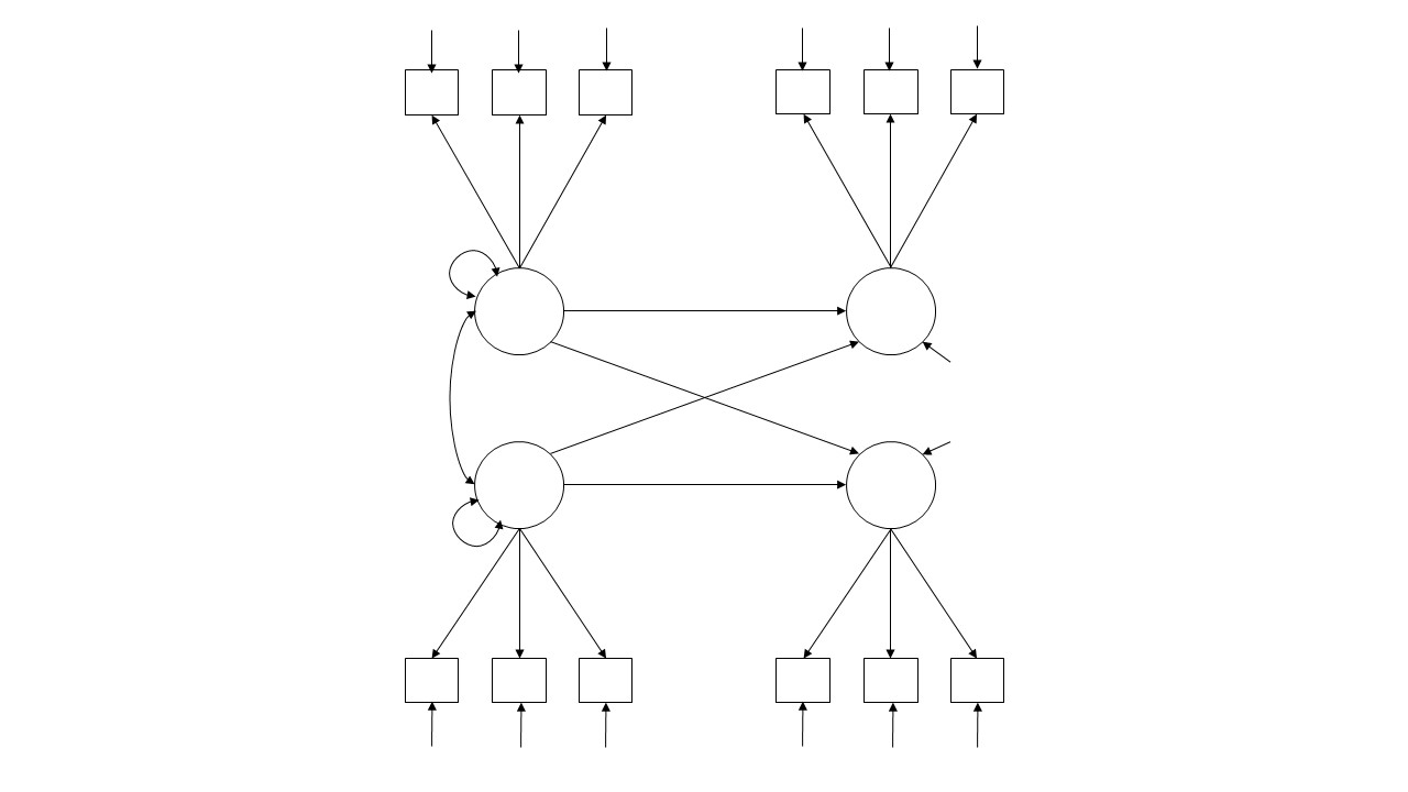
Double-headed arrows are also used to represent the variances (variances and covariances) of exogenous variables. Thus, the covariance of a variable with itself (its variance) is illustrated with a double-headed arrow connecting a variable to itself. Although these are typically omitted from diagrams, it is wise to include them for all exogenous variables when you're initially learning about LVM so you can remember that they represent real parameters about which assumptions must be made in simulations or which must be estimated in empirical applications.

Endogenous variables are rarely fully explained by the structural relations of a model. As such, LVMs almost always include residual terms for endogenous variables. These are often represented as directed arrows and may or may not have a label or symbol.

Tracing Rules

The specific set of structural relations among variables (latent and measured) imply a pattern of covariances or associations among the measured variables. How can we obtain these patterns? Tracing Rules are a commonly used set of guidelines that can be used to express the covariance between any two variables in a path diagram. They were originally proposed by the geneticist, Sewall Wright, in the 1920s.

To find the expected covariance between any two variables, you simply trace all permissible paths between the two variables of interest. The coefficients (path coefficients and variances) along each path are multiplied together; those products are them summed across different tracings or paths. In short, one finds the sum of all compound paths between two variables.

There are a few rules to this tracing game that cannot be violated:

1. Don't spear yourself. You can begin by going backwards against a single-headed arrow. But once you start going forward with the arrows, you can never go against an arrow again.
2. No loops. You cannot go through the variable more than once on a single tracing.
3. One arc. At maximum, you can only go through one double-headed arrow (e.g., a covariance between two exogenous variables) in a single tracing.

Note: When working with standardized variables, the variances are 1. This simplifies the math considerably and allows one to use tracing rules to generate expected correlations among variables. The diagrams in the figure above illustrate the expected correlations among four variables with unit variance (var[x1 - x4] = 1), assuming different causal structures in each case.

Estimating the Parameters LV Models in lavaan

The first step in a lavaan analysis is to specify the core equations for the model. There are three parts to this process, some being more relevant than others depending on the context:

1. Latent variable definitions. The measurement model specifies which measured variables are indicators of which latent variables using the =~ operator.

   	 Examples:
   		LV1 =~ x1 + x2 + x3
   		LV2 =~ x4 + x5 + x6
   
   

2. Regressions. The structural model specifies the linear causal relationships among variables using the ~ operator.

   	Examples:
   		LV3 ~ LV1 + LV2
   		x1  ~ x2
   
   

3. Misc. There are other things that can be done too, such as placing constraints on parameters, freeing constrained parameters, or estimating means/intercepts.

   	 Examples: 
   		x1  ~~ x2	# Allow the residuals for X1 and X2 to correlate
   		LV1 ~~ 1*LV1	# Allow LV1 to covary 1.00 with itself (var = 1)
   		x1  ~1		# Estimate the means/intercepts for x1
   
   

To specify the model in lavaan, one simply creates an object that contains some text that describes the model. There is a formal syntax, of course. Here is an example, but I've left certain parts out that were not necessary (but included some placeholders for future reference). I've used the # symbol liberally to comment the syntax.

	
	model = '
	 # Latent Variable Definitions
	     latent.factor =~ x1 + x2 + x3 + x4
	 # Regressions
	 
	 # Misc
	 '

To estimate the parameters of the model (and evaluate the fit of the model), we use the sem() function in lavaan. In the syntax we specify the model (see above) in question and the data source (preferably a dataframe). We can also use the summary() function to get a nice overview of the results. (Please recall that the lavaan library needs to be loaded for this to work.)

	results = sem(model, data=x)
	summary(results, standardize=TRUE)

Notice that by default lavaan fixed the loading for the first indicator to 1.00. This is done so that there is a scale/metric for the latent variable: the same scale on which x1 is measured is used for the latent factor. (If we prefer, we can set the scale of the latent factor to 1.00 and freely estimate the loadings instead. We will do this below.)

Notice that our loading estimate is not equal to .707; it is 1.00 (on average). Why? When we generated the data, the latent variable had a variance of 1.00. But here we have treated the variance of the latent.factor as a parameter. The estimation procedure compensated accordingly. Notice that the standardized estimates are what we expect; these assume unit variance.

Let's constrain the variance of the latent variable to be 1.00 and, instead, estimate the loadings freely (without using x1 to scale the latent variable).

	model = '
	 # Latent Variable Definitions
	   latent.factor =~ NA*x1 + x2 + x3 + x4

	 # Regressions
	 
	 # Extra
	   latent.factor ~~ 1*latent.factor
	 '
	results = sem(model, data=x)
	summary(results, standardize=TRUE, fit.measures=TRUE)

By pre-multiplying the first indicator by NA, we force lavaan to estimate that parameter rather than use its default assumption that the first loading should be 1.00 to define the scale of the latent variable. Notice that the estimates of the loadings are pretty close to their true value (.707).

lavaan has an alternative method that makes this easier. Specifically, the std.lv=TRUE argument in the sem() call instructs lavaan to standardize the latent variables (lv). When this argument is included, lavaan knows to set the variance of the latent variables to 1.00 and will not longer attempt to scale the latent variable by fixing the loading for the first measure of that factor to 1.00. Here is an example:

	model = '
	 # Latent Variable Definitions
	   latent.factor =~ x1 + x2 + x3 + x4
	 
	 # Regressions
	 
	 # Extra
 	  '
	results = sem(model, data=x, std.lv=TRUE)
	summary(results, standardize=TRUE, fit.measures=TRUE)

Recall that when we generated the data, all the loadings were identical. In this example, we have freely estimated each one. We can see that our estimates are pretty close to one another. But we may wish to impose equality constraints and force lavaan to treat the loadings as a single parameter.

We can do that via a two-step process:

• Create a label: We can create a label for a parameter by pre-multiplying the term by a label of our choosing (e.g., a).
• Identical labels: We pre-multiply all terms that we wish to equate by the same label.

Here is an example where we label the loadings "a" and have a common loading parameter rather than four separate estimates:

	model2 = '
	 # Latent Variable Definitions
	   latent.factor =~ a*x1 + a*x2 + a*x3 + a*x4
	 
	 # Regressions
	 
	 # Extra
 	  '
	results2 = sem(model2, data=x, std.lv=TRUE)
	summary(results2, standardize=TRUE, fit.measures=TRUE)

Note: Because the model with equality constraints is nested within the model that allowed those loadings to vary freely, we can test the extent to which this equality constraint impairs the fit of the model. We can do this using the anova() function, placing the results objects in the arguments. This will show the AIC and BIC for the two models and provide a chi-square diff test for the two models.

	anova(results, results2)

According to our output, the fit of the model is not significantly impaired by assuming equal loadings. Moreover, imposing this constraint made free 3 additional degrees of freedom.

Using a Covariance Matrix as Input Rather Than Raw Data

In the examples above, we used the data = x argument in the sem() command to specify the data frame of interest. Sometimes it is useful to use the var-cov matrix rather than the raw data as input. For example, the var-cov info is often published in articles (or the cor matrix with SDs), even if the raw data are not. By using this info as the 'input' for lavaan, you can attempt to reproduce the results of other researchers or examine alternative models that might be of interest to you that were not examined in the original report.

There are several ways to read in the var-cov matrix. One simple way is to use the getCov() function in lavaan. This function accepts as input the lower diagonal of a matrix. You can also name the variables. Here is an example:

	lower = '
	 9.060 
	 6.567 9.181 
	 5.760 5.708 8.940 
	 4.436 4.203 3.197 8.352 
	 3.319 3.431 3.386 3.273 8.880 '

	wisc.cov = getCov(lower, names = c("Information", "Similarities", 
	"Word.Reasoning", "Matrix.Reasoning", "Picture.Concepts"))

	wisc.cov

(These data and some of the examples come from Alexander Beaujean's book, 'Latent Variable Modeling Using R'. Highly recommended!)

You can also input a correlation matrix and, if you have access to the SDs of the variables too, turn that matrix into a var-cov matrix.

	# Let's first input the cor matrix

	lower = '
	 1.00 
	 0.72 1.00 
	 0.64 0.63 1.00 
	 0.51 0.48 0.37 1.00 
	 0.37 0.38 0.38 0.38 1.00 '

	wisc.cor = getCov(lower, names = c("Information", "Similarities", 
	"Word.Reasoning", "Matrix.Reasoning", "Picture.Concepts"))

	wisc.cor

	# Convert cor matrix to cov using cors and SDs

	wisc.cov = cor2cov(R = wisc.cor, sds = c(3.01, 3.03, 2.99, 2.89, 2.98))
	wisc.cov

The cor2cov() function allows us to transform a correlation matrix into a covariance matrix (but we have to also supply the SDs for the variables). There is also a handy function in lavaan called cov2cor() that transforms a covariance matrix into a correlation matrix.

Once you have objects that contain the var-cov matrix, you can adjust the sem() call in the following way to specify the var-cov matrix as input rather than the raw data file:

	sem(model1, sample.cov=wisc.cov, sample.nobs=550)

Not only do you need to specify the object name for the var-cov matrix, you also have to indicate the sample size.

Confirmatory Factor Analysis (CFA) and Basic Factor Models

Let's do some basic factor analysis using the wisc data from above.

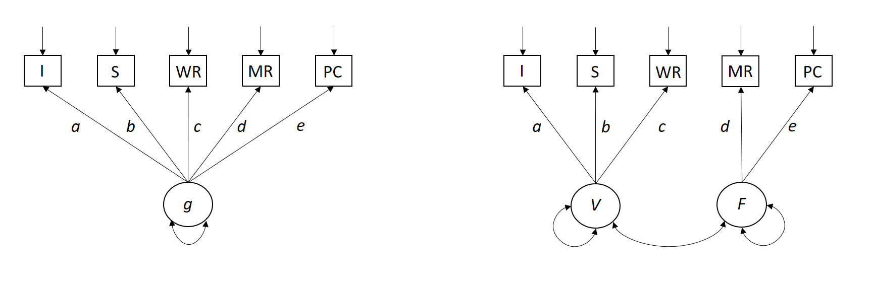
Let's begin by estimating the parameters of a single-factor model. We will label the common factor 'g' because we are creative. Our model states that there is a latent variable, g, that gives rise to variation in the five cognitive tests that were administered (see the left-panel of the figure below). We have also provided labels for the loading parameter estimates to make it easier to see how elements of the output map onto the picture on the board.

	model1 = '
		#Latent Variable Definitions
		  g =~ a*Information + b*Similarities +
			c*Word.Reasoning + d*Matrix.Reasoning +
			e*Picture.Concepts'

	results = sem(model1, sample.cov=wisc.cov, sample.nobs=550)
	summary(results,standardized = TRUE, fit.measures=TRUE)

Please note that I've introduced a new feature here: fit.measures=TRUE. This instructs lavaan to provide a detailed list of commonly used fit measures in SEM work. We can see even more indices if we type in:

	fitMeasures(results)
	

Notice that lavaan automatically used the first measured variable to scale the latent variable. As discussed above, this is the default behavior of lavaan when latent variables are defined. We can change this default if we wish by explicitly freeing that parameter (NA) and constraining the variance of g to be 1.00 (g ~~ 1*g).

	model2 = '
		#Latent Variable Definitions
		  g =~ NA*Information + b*Similarities +
		     c*Word.Reasoning + d*Matrix.Reasoning +
		     e*Picture.Concepts
     		# Misc
		  g ~~ 1*g
	     '

	results2 = sem(model2, sample.cov=wisc.cov, sample.nobs=550)
	summary(results2,standardized = TRUE, fit.measures=TRUE)

We can also use the std.lv=TRUE option in the sem() call. Doing so constrains the variance of the latent variable to be 1.00 and, thereby, allows us to estimate the loading for the first measured variable rather than using it to scale the latent variable.

	model2b = '
		#Latent Variable Definitions
		  g =~ a*Information + b*Similarities +
		     c*Word.Reasoning + d*Matrix.Reasoning +
		     e*Picture.Concepts
		'

	results2b = sem(model2b, sample.cov=wisc.cov, sample.nobs=550,
		std.lv=TRUE)
	summary(results2b,standardized = TRUE, fit.measures=TRUE)

Although a one-factor model appears to fit these data well, it is valuable to consider alternative model specifications. One alternative is that there are two (highly correlated) factors underlying these data. For example, there may be a Verbal Comprehension (V) factor giving rise to the first three measures and a Fluid Reasoning (F) factor giving rise to the other two. We can examine this possibility by defining two latent factors, V and F.

	model3a<-'
		#Latent Variable Definitions
		 V =~ a*Information + b*Similarities + c*Word.Reasoning 
		 F =~ d*Matrix.Reasoning + e*Picture.Concepts

		# Misc
		 V ~~ f*F
	'

	results3a = sem(model3a, sample.cov=wisc.cov, sample.nobs=550, std.lv=TRUE)
	summary(results3a,standardized = TRUE, fit.measures=TRUE)

This model fits the data well too. But they are not directly comparable because they involve different latent structures (e.g., varying numbers of latent variables).

One way to nest them is to compare this model against one that assumes the two factors are perfectly related. This is comparable to testing a one- vs. a two-factor model (see the right-hand panel of the figure above). To do this, let's again define two latent variables, but fix the covariance between V and F to be 1 (V ~~ 1*F).

	model3b<-'
		#Latent Variable Definitions
		  V =~ a*Information + b*Similarities + c*Word.Reasoning 
		  F =~ d*Matrix.Reasoning + e*Picture.Concepts

		 # Misc
		  V ~~ 1*F
	'

	results3b = sem(model3b, sample.cov=wisc.cov, sample.nobs=550, std.lv=TRUE)
	summary(results3b,standardized = TRUE, fit.measures=TRUE)

We can compare the fit of these two models using the anova() function.

	anova(results3a, results3b)

The results suggest that imposing the equality constraint (i.e., defining the two factors as being perfectly related to each other) significantly impaired the fit of the model. Thus, a two-factor solution might be preferable, despite the high correlation (.82) between the two factors.

Measurement Models and Measurement Invariance

A common application of LVM for measurement purposes is for the assessment of various measurement models. Measurement is a core part of what we do in psychology. And, as such, we need methods for evaluating our measurement models so that we can assure that we are assessing the constructs we intend to assess and that we are scaling people appropriately.

To illustrate some of these applications in R, I'll draw upon some data on the reliability of essay writing scoring. The data come from an examination of reader reliability in essay scoring among 126 examinees. Four versions of the essays were scored:

• orig1 = the original essay part 1
• hwcpy1 = a hand-written copy of orig1
• ccpy1 = a carbon copy of hwcpy1
• orig2 = the original essay part 2

Thus, there are four measured variables in our example. The example and data come from Seppo Pynnönen.

Let's read in the var-cov matrix for the data.

	lower = '
	25.0704
	12.4363 28.2021
	11.7257 9.2281 22.7390
	20.7510 11.9732 12.0692 21.8707'

	m.cov = getCov(lower, names = c("orig1", "hwcpy1","ccpy1","orig2"))
	m.cov

We assume from the outset that these four measures are, in fact, measures of a common construct: essay writing skillz. Thus, it is sensible to assume that there is a common latent factor underlying them. Nonetheless, we could test this assumption using some of the methods described above. (We'll skip this for now, however.)

One of the big questions we wish to address is whether the four tests are equally good measures of the construct they are supposed to assess. We want to know this for many reasons. If, for example, one of the tests is a poorer measure of skillz than the others, we may wish to discard scores from that test or discontinue or improve its use.

• Parallel Tests

  Let's begin by assuming that the four tests are equally good measures of the latent trait. The assumption of "parallel tests" in classical test theory is that the various tests have equal true score variances AND equal error variances. This is a strict set of assumptions. If they don't hold well, we can begin to relax them to refine the measurement model.

  In a LVM framework, we can evaluate these assumptions by (a) assuming a common latent trait (true scores) and equating the loadings and (b) equating the measured residuals.

  
  		model.par = '
  			#Latent Variable Definitions
  			  true =~ a*orig1 +
  				  a*hwcpy1 +
  				  a*ccpy1 + 
  				  a*orig2 
  
  			# Misc
  				orig1  ~~ b*orig1
  				hwcpy1 ~~ b*hwcpy1
  				ccpy1  ~~ b*ccpy1
  				orig2  ~~ b*orig2
  		     '
  
  		results.par = sem(model.par, std.lv=TRUE, sample.cov=m.cov, sample.nobs=126)
  		summary(results.par,standardized = TRUE)
  		
  

  Note that this model does not fit the data well.

• Tau Equivalence

  Let's relax the assumption that the error variances are the same across tests.

  Measures are considered tau equivalent if their true score variances are the same. This is comparable to assuming that the loadings for each test on the latent factor are identical. There is no assumption that the error variances are the same.

  
  		model.tau = '
  			#Latent Variable Definitions
  			  true =~ a*orig1 +
  				  a*hwcpy1 +
  				  a*ccpy1 + 
  				  a*orig2 
  			# Misc
  		     '
  
  		results.tau = sem(model.tau, std.lv=TRUE, sample.cov=m.cov, sample.nobs=126)
  		summary(results.tau,standardized = TRUE)
  		
  

  This model does not fit as poorly as the Parallel Tests model.

• Congeneric

  Measures are considered congeneric if their true scores correlate perfectly with each other. This is comparable to stating that the measures are caused by a common latent factor. However, there is no assumption that the loadings are the same. Nor is there an assumption that the residual variances are the same across measures. In short, we are assuming that the same true scores are measured by the four tests. But each test has a different relationship to the true scores than the other tests. And some have more errors than the others.

  
  		model.con = '
  			#Latent Variable Definitions
  			  true =~ a*orig1 +
  				  b*hwcpy1 +
  				  c*ccpy1 + 
  				  d*orig2 
  			# Misc
  		     '
  
  		results.con = sem(model.con, std.lv=TRUE, sample.cov=m.cov, sample.nobs=126)
  		summary(results.con,standardized = TRUE)
  		
  

Compare models and estimate reliability

Each of these measurement models are nested within the more inclusive congeneric model. As such, we can compare their relative fit to the data using the anova() function:

		anova(results.con,results.tau,results.par)

We see here that the congeneric model provides the best fit to the data. Each set of assumptions that we add to it (e.g, equal loadings) significantly impairs the fit of the model to the data. This implies that, although the various tests may be measures of the same latent construct, they are not equivalent measures of that construct. Some may be better than others.

We can estimate reliability within this framework. Reliability is defined as the proportion of true score variance relative to the observed score variance. In the examples above we constrained the variance of the true scores to 1.00. Thus, the square of the factor loading represents the true score variance. If we divide this by the total score variance, we have an estimate of reliability of each measure.

We can extract the parameter estimates using the coef() function in lavaan. We can use these estimates to compute reliability under the assumptions of each measurement model.

		loadings = coef(results.con)[1:4]
		resid.var = coef(results.con)[5:8]
		loadings^2 / (loadings^2 + resid.var)

		loadings = coef(results.tau)[1:4]
		resid.var = coef(results.tau)[5:8]
		loadings^2 / (loadings^2 + resid.var)

		loadings = coef(results.par)[1:4]
		resid.var = coef(results.par)[5:8]
		loadings^2 / (loadings^2 + resid.var)

Measurement Equivalence Across Groups

A common research question in psychological science concerns differences between groups. For example, we may have measured a psychological trait of interest (e.g., depression) and be concerned with sex differences, cultural differences, or age group differences.

The typical way of addressing this issue is to compute the mean difference between groups and test it with a t-test (or some other statistical model). If the difference is statistically significant, we conclude that the two groups differ with respect to the psychological trait of interest.

One of the limitations of this approach, however, is that it assumes that the measurement instrument works in the same way for the two groups. It assumes, for example, that men and women interpret and use the items in the same way.

Why does this matter? If the construct of interest is not being measured in the same way across groups, then observed group differences could be due to differences in the measurement process itself rather than true (i.e., latent variable) differences. Until we have demonstrated that the measures assess the same construct across the two groups, we can not confidently draw conclusions about the source of observed differences.

There are many ways to study measurement equivalence or measurement invariance in modern psychology. One method involves using latent variable models. The approach holds that measures across groups are considered to be on the same scale if relationships between the indicators and the latent trait are the same across groups. But invariance isn't an all or none state. As we discuss below, there are strong and weak forms of invariance.

Notice that we have not discussed means up until this point. Many applications of latent variable modeling focus only on covariance structures. In these applications, the means are typically not of interest. (In fact, the means are independent of the covariance structure.)

LVMs, however, can incorporate means or mean structures. In path diagrams, means are incorporated by including a triangle--a constant of 1. The mean of a latent variable is alpha * 1 (i.e., the constant). The mean of a measured variable becomes a function of both the mean of the latent variable(s) that causes it and the item intercept. These means can be computed using the same kinds of tracing methods described before (summing compound paths), with two new rules. One starts with the measured variable and traces the paths to the constant. There are two new tracing rules that apply when finding means: (1) the paths can only go through directional arrows; they cannot go through bidirectional arrows and (2) the paths can only go backwards along arrows; one cannot move forward along an arrow.

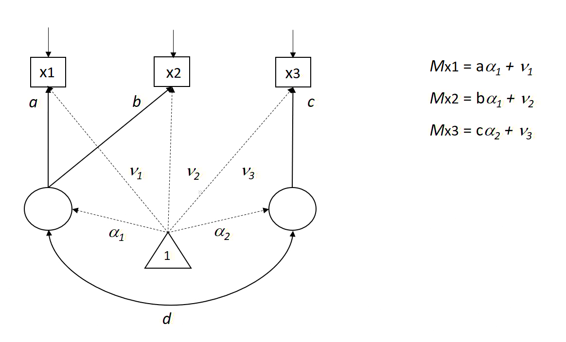
In a LVM framework, the means for measured variables can be decomposed into three components:

Mean[measured] = nu + lambda*alpha

1. nu. The intercepts of the measured variables.
2. alpha. The mean of the latent variables/factors/traits.
3. lambda. The loadings of the measured variables on the latent factors.

This formalism makes it clear that mean differences can be due to any of these factors. Two groups can differ from one another because they have different intercepts (use the scale differently), the mapping between the measure and the latent trait are not the same, or the two groups really differ on the latent variable. To evaluate the later (the part we typically care about), we want to rule out the other two.

Measurement equivalence is typically appraised in a series of steps that impose ever more stringent restrictions.

1. Configural Invariance.

This assumes that the core measurement model is the same for the two groups. That is, the same number of latent variables exist. There is no assumption, however, that the loadings are the same or that anything else is the same. This model implies that similar, but not necessarily identical, latent variables are present across the groups. This model serves as a useful baseline against which we can compare more restrictive models.

2. Weak Invariance (Factorial Invariance).

In this model we constrain the factor loadings (lambda) to be equivalent across groups. This implies that the same latent variables are being measured in both groups.

An implication of this model is that differences in the covariances between variables across groups are due to differences in the covariances of the latent variables. This is kind of cool, even if it isn't our main concern right now.

If a Weak Invariance model fits as well as a Configural Invaraince model, one might be justified in assuming that the measurement model is the same for the two groups.

3. Strong Invariance.

In this model we constrain both lambda and nu (i.e., the intercepts of the measured variables) across the two groups. This is often called strong invariance.

When a strong invariance model fits the data reasonably well, one can examine the latent means (alpha) to see if they differ between groups. Because the intercepts (and the measurement model) are constrained to be the same across the two groups, the differences in means cannot be explained easily by these factors.

Example:

Lavaan has a few different ways to deal with multiple group structures. If you are working with the raw data, for example, you can use the group = "x" argument to indicate the grouping variable.

I'll illustrate some of these ideas using a dataset built into lavaan. This dataset contains cognitive measurements on children at two different schools (Pasteur and Grant-White).

Let's begin with configural invariance to establish a baseline model.

	HS.model <- '  
		visual  =~ x1 + x2 + x3
		textual =~ x4 + x5 + x6
		speed   =~ x7 + x8 + x9 
	'

	fit1 = sem(HS.model, 
		   data = HolzingerSwineford1939, 
		   group = "school")
	summary(fit1)

(Note: We can't estimate all the possible parameters freely because there is not enough information. In this analysis, lavaan is automatically setting the means of the latent variables to 0.00. Without further constraints, the latent means cannot be estimated. Fortunately, the values of the latent means are not relevant for evaluating configural invariance.)

Next, let's constrain the loadings to be the same across groups and see how that impacts the fit to the data. (Note. We do not need to input the model statement again; it is the same across the examples that follow.)

	fit2 = sem(HS.model, 
		   data = HolzingerSwineford1939, 
		   group = "school",
		   group.equal = c("loadings")
		   )
	summary(fit2)

	anova(fit1, fit2)

In this case, the fit of the two models is close enough. We can assume that the tests are measuring the same constructs across the two groups. But we can get more nuanced if we wish:

Let's equate the intercepts too:

	fit3 = sem(HS.model, 
		   data = HolzingerSwineford1939, 
		   group = "school",
		   group.equal = c("loadings", "intercepts")
		   )
	summary(fit3,standardized = TRUE)

	anova(fit2, fit3)

This change leads to a significant change in model misfit. Requiring the intercepts to be the same across the two groups impairs to some degree our ability to model the data accurately.

lavaan estimates the latent mean differences between the two groups by fixing the latent means to zero for the first group and estimating the means for the second group. Notice that two of these means are statistically significant. This model suggests that there are textual differences between the two groups even when you equate the intercepts across the groups.

Please note that you can equate many parameters across groups. You can even examine partial invariance by equating certain sets of parameters (e.g., loadings), but freeing specific ones. For more information on your options, please see the lavaan website.

Bifactor Models

Bifactor models are often used to partition variance in specific ways. They are not necessarily used to test or recover latent factor structures, although they can be used for that purpose too.

There are two key ingredients in bifactor models:

1. The latent factors are constrained to be uncorrelated with one another.
2. All the measurements are regressed on a common factor. The remaining factors (sometimes called group factors) predict only subsets of measurements.

One of the advantages of working with bifactor models is that they have the potential to allow one to study factors with greater 'purity.' If there is a general factor present, then it potentially confounds any estimated association between predictors and outcomes. By isolating the general factor, one can zoom-in on the parts that matter. In some cases, the general factor may be of substantive interest.

This model structure is easy to implement in lavaan. Here is an example using the WISC data we've used already. (I've repasted the data below.) We will retain the same factors we used before. But, in addition to those, we will add a factor, g, that is related to all the measurements. We will also impose the constraint that all latent variables be uncorrelated using the orthogonal=TRUE statement in the sem() function. This is a compact alternative to writing out a bunch of g ~~ 0*Information, g ~~ 0*Similarities, etc. statements.

	
	# Data
	lower = '
	 9.060 
	 6.567 9.181 
	 5.760 5.708 8.940 
	 4.436 4.203 3.197 8.352 
	 3.319 3.431 3.386 3.273 8.880 '

	wisc.cov = getCov(lower, names = c("Information", "Similarities", 
	"Word.Reasoning", "Matrix.Reasoning", "Picture.Concepts"))

	wisc.cov

	# Model

	# This is a bifactor model with equality constraints
	# to enable identification (too many free parameters otherwise)

	wisc.bifac.model1 <- '
		g	=~ a*Information + a*Similarities + a*Word.Reasoning + a*Matrix.Reasoning + a*Picture.Concepts

		f1  =~ Information + Similarities + Word.Reasoning 
		f2  =~ Matrix.Reasoning + Picture.Concepts
	'


	fit1 = sem(wisc.bifac.model1, 
		   sample.cov = wisc.cov, 
		   sample.nobs = 550,
		   orthogonal=TRUE, 
		   std.lv = TRUE
		   )
	summary(fit1,standardized = TRUE, fit.measures=TRUE)

This model appears to fit the data well. Notice that the loading for Matrix.Reasoning flips sign in the bifactor model. This seems a bit odd and would require careful inspection if we were conducting substantive research in this area. It might be a quirk of a mispecified model. But it might also reveal suppression.

As another example, let's examine data on basic personality traits. The following dataset is from one of my studies and contains measures of the IPIP 20 from approximately 48,000 people. There is also a self-report measure of general health (health01): "In general, would you say your health is" rated on a 1 (poor) to 5 (excellent) scale. Let's use the bifactor model to extract a general factor and see how that and the other personality factors are related to health.

	# read in data from internet
	ipip2 = read.table("http://yourpersonality.net/R Workshop/ipip2.txt",
		header=TRUE, sep=",")


	ipip.model <- '
		g =~ vipip01 + vipip02 + vipip03 + vipip04 + vipip05 + 
		     vipip06 + vipip07 + vipip08 + vipip09 + vipip10 + 
		     vipip11 + vipip12 + vipip13 + vipip14 + vipip15 + 
		     vipip16 + vipip17 + vipip18 + vipip19 + vipip20  

		e =~ vipip01 + vipip02 + vipip03 + vipip04
		a =~ vipip05 + vipip06 + vipip07 + vipip08
		c =~ vipip09 + vipip10 + vipip11 + vipip12
		n =~ vipip13 + vipip14 + vipip15 + vipip16
		o =~ vipip17 + vipip18 + vipip19 + vipip20
	'

	ipip.model.fit <- sem(ipip.model, data = ipip2, orthogonal=TRUE, std.lv = TRUE) 
	summary(ipip.model.fit, fit.measures = TRUE, standardized = TRUE)

Notice that this model doesn't fit the data well, although it is not awful. The more troubling part is that one of the residual errors is negative, which indicates that something is not "right" with the model.

Although it takes us slightly off topic, I'll show you a lavaan trick that can be helpful in situations like this. Specifically, we can impose a constraint on the estimation process. I've added two new lines below. The first labels the residual variance for vipip17. We have labeled the parameter 'a'. The second line states that a must be larger than 0. The inclusion of this constraint allows the model to run without error. It is important to note that we haven't solved the problem; we've merely created a band-aid. If our model were appropriate, we wouldn't need this kind of adjustment.

	ipip.model <- '
		g =~ vipip01 + vipip02 + vipip03 + vipip04 + vipip05 + 
		     vipip06 + vipip07 + vipip08 + vipip09 + vipip10 + 
		     vipip11 + vipip12 + vipip13 + vipip14 + vipip15 + 
		     vipip16 + vipip17 + vipip18 + vipip19 + vipip20  

		e =~ vipip01 + vipip02 + vipip03 + vipip04
		a =~ vipip05 + vipip06 + vipip07 + vipip08
		c =~ vipip09 + vipip10 + vipip11 + vipip12
		n =~ vipip13 + vipip14 + vipip15 + vipip16
		o =~ vipip17 + vipip18 + vipip19 + vipip20

		# Constraint to ensure the resid var is > 0
		vipip17 ~~ a*vipip17
		a > 0.001
	'

	ipip.model.fit <- sem(ipip.model, data = ipip2, orthogonal=TRUE, std.lv = TRUE) 
	summary(ipip.model.fit, fit.measures = TRUE, standardized = TRUE)

Although the model fit is not great, that might not be due to the assumption of a general bifactor. It may be due to the strict assumption of orthogonal latent variables.

Let's unpack this first by removing the general factor. We can do so by fixing the weights to 0. This allows the two models to be nested so we can compare their fits more naturally.

	ipip.model2 <- '
		g =~ 0*vipip01 + 0*vipip02 + 0*vipip03 + 0*vipip04 + 0*vipip05 + 
		     0*vipip06 + 0*vipip07 + 0*vipip08 + 0*vipip09 + 0*vipip10 + 
		     0*vipip11 + 0*vipip12 + 0*vipip13 + 0*vipip14 + 0*vipip15 + 
		     0*vipip16 + 0*vipip17 + 0*vipip18 + 0*vipip19 + 0*vipip20  

		e =~ vipip01 + vipip02 + vipip03 + vipip04
		a =~ vipip05 + vipip06 + vipip07 + vipip08
		c =~ vipip09 + vipip10 + vipip11 + vipip12
		n =~ vipip13 + vipip14 + vipip15 + vipip16
		o =~ vipip17 + vipip18 + vipip19 + vipip20

		# Constraint to ensure the resid var is > 0
		vipip17 ~~ a*vipip17
		a > 0.001
	'

	ipip.model.fit2 <- sem(ipip.model2, data = ipip2, orthogonal=TRUE, std.lv = TRUE) 
	summary(ipip.model.fit2, fit.measures = TRUE, standardized = TRUE)

	anova(ipip.model.fit,ipip.model.fit2)

The fit is a bit worse without the assumption of a general factor. So let's hold onto that idea and, next, relax the assumption that the personality traits are orthogonal. We will, however, force the general factor to be orthogonal to the personality traits.

	ipip.model3 <- '
		g =~ vipip01 + vipip02 + vipip03 + vipip04 + vipip05 + 
		     vipip06 + vipip07 + vipip08 + vipip09 + vipip10 + 
		     vipip11 + vipip12 + vipip13 + vipip14 + vipip15 + 
		     vipip16 + vipip17 + vipip18 + vipip19 + vipip20  

		e =~ vipip01 + vipip02 + vipip03 + vipip04
		a =~ vipip05 + vipip06 + vipip07 + vipip08
		c =~ vipip09 + vipip10 + vipip11 + vipip12
		n =~ vipip13 + vipip14 + vipip15 + vipip16
		o =~ vipip17 + vipip18 + vipip19 + vipip20

		g ~~ 0*e
		g ~~ 0*a
		g ~~ 0*c
		g ~~ 0*n
		g ~~ 0*o

		# Constraint to ensure the resid var is > 0
		vipip17 ~~ a*vipip17
		a > 0.001
	'

	ipip.model.fit3 <- sem(ipip.model3, data = ipip2, orthogonal=FALSE, std.lv = TRUE) 
	summary(ipip.model.fit3, fit.measures = TRUE, standardized = TRUE)
	
	anova(ipip.model.fit3,ipip.model.fit2)

This improves the fit. Thus, if we wanted to optimally model the covariance structure for these data, we would want to allow covariation among the latent traits. But, in the spirit of bifactor models, let's again force the latent variables to be orthogonal.

In addition, let's now investigate the association between health and (a) the general factor and (b) personality traits 'purged' of the general factor.

	ipip.model <- '
		g =~ vipip01 + vipip02 + vipip03 + vipip04 + vipip05 + 
		     vipip06 + vipip07 + vipip08 + vipip09 + vipip10 + 
		     vipip11 + vipip12 + vipip13 + vipip14 + vipip15 + 
		     vipip16 + vipip17 + vipip18 + vipip19 + vipip20  

		e =~ vipip01 + vipip02 + vipip03 + vipip04
		a =~ vipip05 + vipip06 + vipip07 + vipip08
		c =~ vipip09 + vipip10 + vipip11 + vipip12
		n =~ vipip13 + vipip14 + vipip15 + vipip16
		o =~ vipip17 + vipip18 + vipip19 + vipip20

		# Constraint to ensure the resid var is > 0
		vipip17 ~~ a*vipip17
		a > 0.001

		# Regression health on all latent vars
		health01 ~ g + e + a + c + n + o
	'

	ipip.model.fit <- sem(ipip.model, data = ipip2, orthogonal=TRUE, std.lv = TRUE) 
	summary(ipip.model.fit, fit.measures = TRUE, standardized = TRUE)

Notice that most the regressions of health are significantly related to the latent variables. (The sample size is large.) Some of the associations are > .10 in a standardized metric. C is positively related to Health; N is negatively related to Health. (The latent traits may be estimated in the direction opposite the trait label. Interpret the associations appropriately. When I ran this, what I labeled "c" was actually low c.)

Of note: These associations exist after controlling for whatever variance is common to all the items. Also, whatever that common factor is, it also inversely predicts health.

Mediation

Let's explore next a simple path model of the mediation variety:

x --> m --> y

Let's begin by generating the data ourselves so we know the true parameters. We will then see whether lavaan can recover those accurately.

	n = 10000
	ba = .2
	bb = .4
	bc = .0

	x = rnorm(n)
	m = ba*x + rnorm(n)
	y = bb*m + bc*x + rnorm(n)

	x = cbind(x,m,y)
	x = data.frame(x)
	cor(x)

Now, let's specify the model of interest using the lavaan syntax and run the sem() function.

	model = '
	 # Latent Variable Definitions

	 # Regressions
	   m ~ a*x
	   y ~ b*m + c*x
	 
	 # Extra
	   ab := a*b
	 '
	results = sem(model, data=x)
	summary(results, standardize=TRUE, fit.measures=TRUE)

I have added an extra model statement to the syntax to illustrate another lavaan trick. Namely, one can define a new parameter using the := operator. In this situation, we have defined a new parameter called 'ab' which we have set to equal the product of paths a and b. This is a test of the indirect effect of x on y through m. And, once we define it, we can test the coefficient and see whether it is significantlly different from 0. (It is in this case.)

Multiple Regression Using FIML

We had previously learned how to use the lm() function in R to estimate the parameters of a multiple regression model. One of the limitations of that procedure is that it does not handle missing data well. Specifically, it defaults to listwise methods. One of the powerful features of lavaan is that it allows for a number of estimation methods to be used, including full information maximum liklihood methods. Many people consider the use of ML methods to be 'best practice' at the moment.

We can use ML estimation in lavaan to estimate the parameters of a classic multiple regression model with missing data. Here in an example, drawing upon one we used previously:

	n = 300
	r = .3
	x1 = rnorm(n)
	x2 = r*x1 + rnorm(n,0,sqrt(1-r^2))
	cor(x1,x2)
	b1 = .2
	b2 = .3
	y = 10 + b1*x1 + b2*x2 + rnorm(n,0,sqrt(1 - ((b1^2) + (b2^2) + (2*b1*b2*r))))

Notice that if we run lm() on this complete data set, we won't have any problems. And, with a sample size of 300 or so, we have have reasonably accurate estimates of the model parameters.

	summary(lm(y ~ x1 + x2))

Now let's add missing values at random to the predictors:

	k = 100				# number of missing values

	x.full = x.missing = data.frame(cbind(y, x1, x2))

	for (i in 1:k) {
	  this.case = sample(1:n)[1]	# select a case at random
	  this.var = sample(2:3)[1]	# select a variable at random
	  x.missing[this.case, this.var] = NA
	}

	sum(is.na(x.missing))		# how many missing

Run the regression analyses on the complete set of data (x.full) and the on the data set that contains missing values (x.missing)

	summary(lm(y ~ x1 + x2, data = x.full))
	summary(lm(y ~ x1 + x2, data = x.missing))

Notice that the output statement for the second regression says something like "(83 observations deleted due to missingness)." R is using casewise/listwise deletion and analyzing the cases for which full data exist.

Now let's use lavaan for multiple regression. Let's begin by writing the model statement. Most of this should be straight-forward at this point. But please note that we must include y ~ 1 if we want lavaan to estimate the intercept for y.

	model <- ' 
		# Latent Variable Definitions

		# Regressions
		  y ~ x1 + x2 
		# Misc
		  y ~ 1
	'

Let's first analyze the data for the full dataset and verify that the results we get are the same as what we get using the lm() function.

	fit <- sem(model, data = x.full)
	summary(fit, standardized = TRUE, rsquare = TRUE)

This checks out. Note also that I added two useful features to the summary() call. Specifically, I requested a standardized solution so that we can see the unstandardized regression weights (sometimes called B values) and the standardized regression weights (sometimes called beta values).

I also requested r-square.

Let's see what happens with the missing data set.

	fitm <- sem(model, data = x.missing)
	summary(fitm, standardized = TRUE, rsquare = TRUE)

This is similar to what we saw with lm(). The analysis is based on 217 cases (or something similar; there is randomness in the data generation simulation) rather than the full 300.

We can instruct lavaan to use Full Information Maximum Liklihood (FIML) using the missing = "ML" or missing = "FIML" arguments.

	fitm <- sem(model, data = x.missing, missing = "ML")
	summary(fitm, standardized = TRUE, rsquare = TRUE)

Now lavaan uses all the information it has available to estimate the parameters. Notice that the standard errors are a bit smaller with FIML than they were in the example in which listwise deletion was used.

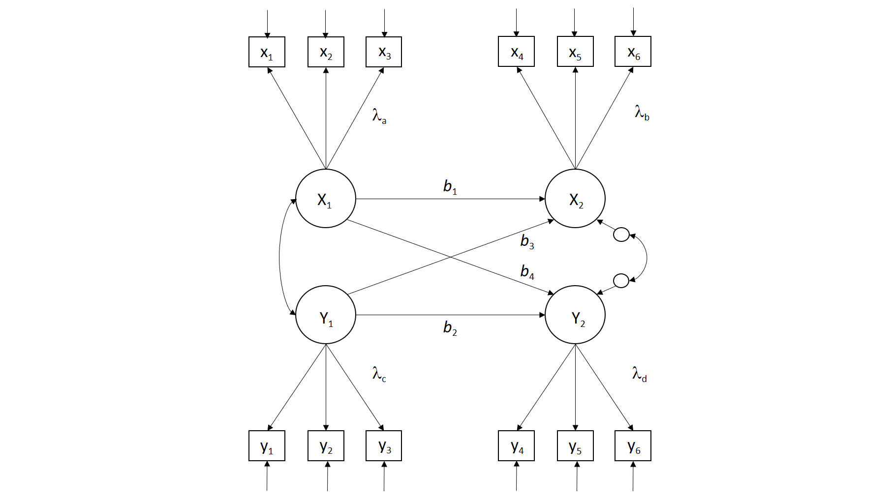
A Longitudinal Two-Wave Panel Model

Many psychologists are interested in studying the associations between person-based variables (e.g., traits, abilities, motives) and contextual/situational factors or performance outcomes (e.g., quality of parenting, peer rejection, job performance). When these associations are examined across time on two occassions, the model used is often a cross-lagged panel model (see the figure below). This model assumes that the two constructs of interest exhibit some degree of stability over time (b1 and b2). Moreover, there is an assumption that the two constructs may cause each other over time (b3, b4).

There are many scholars who question whether this model accurately captures the assumptions we tend to hold about change, development, causation, etc. But I'll discuss it here because (a) it provides a way for us to build on now familiar ideas using a different example, (b) it allows us to more fully illustrate a complex SEM model with measurement and structural components, and (c) it is still commonly used in the psychological literature.

First, let's generate data from a known model.

	# Basic parameters of the model

	 n = 50000		# sample size
	 r = .3			# exogenous correlation between X1 and Y1

	 b1 = .7		# regression of X2 on X1 (stability)
	 b2 = .7		# regression of Y2 on Y1 (stability)
	 b3 = .3		# regression of X2 on Y1 (cross)
	 b4 = .0		# regression of Y2 on X1 (cross)

	 la = .8		# loading of x1-x3 on X1
	 lb = .8		# loading of x4-x6 on X2
	 lc = .8		# loading of y1-y3 on Y1
	 ld = .8		# loading of y4-y6 on Y1

	# Generate X1 from random normal
	# and generate Y1 to correlate r with X1

	 X1 = rnorm(n)
	 Y1 = r*X1 + rnorm(n,0,sqrt(1-r^2))

	# Generate X2 and Y2
	# Both are a function of themselves over time and each other

	 X2 = b1*X1 + b3*Y1 + rnorm(n,0,sqrt(1 - ((b1^2) + (b3^2) + (2*b1*b3*r))))
	 Y2 = b2*Y1 + b4*X1 + rnorm(n,0,sqrt(1 - ((b2^2) + (b4^2) + (2*b2*b4*r))))

	# Generate measured variables as function of latents

 	 x1 = la*X1 + rnorm(n, 0, sqrt(1 - la^2))
	 x2 = la*X1 + rnorm(n, 0, sqrt(1 - la^2))
	 x3 = la*X1 + rnorm(n, 0, sqrt(1 - la^2))

	 x4 = lb*X2 + rnorm(n, 0, sqrt(1 - lb^2))
	 x5 = lb*X2 + rnorm(n, 0, sqrt(1 - lb^2))
	 x6 = lb*X2 + rnorm(n, 0, sqrt(1 - lb^2))

	 y1 = lc*Y1 + rnorm(n, 0, sqrt(1 - lc^2))
	 y2 = lc*Y1 + rnorm(n, 0, sqrt(1 - lc^2))
	 y3 = lc*Y1 + rnorm(n, 0, sqrt(1 - lc^2))

	 y4 = ld*Y2 + rnorm(n, 0, sqrt(1 - ld^2))
	 y5 = ld*Y2 + rnorm(n, 0, sqrt(1 - ld^2))
	 y6 = ld*Y2 + rnorm(n, 0, sqrt(1 - ld^2))

	# Collect measured variables and place them
	# in a dataframe for analysis

	 x = cbind(x1,x2,x3,x4,x5,x6,y1,y2,y3,y4,y5,y6)
	 x = data.frame(x)

	# Let's check and see if the latents are correlated
	# as expected

	 round(cor(cbind(X1,X2,Y1,Y2)),2)

Now, let's build a model statement in lavaan and then use the sem() function to estimate the parameters.

	model <- '
	   # Latent Variable Definitions
		X1 =~ x1 + x2 + x3
		X2 =~ x4 + x5 + x6

		Y1 =~ y1 + y2 + y3
		Y2 =~ y4 + y5 + y6

	   # Regressions
		X2 ~ b1*X1 + b3*Y1
		Y2 ~ b2*Y1 + b4*X1

	   # residual covariances
		X1 ~~ Y1
		X2 ~~ Y2
	'

	results = sem(model, data=x)
	summary(results,standardized = TRUE, fit.measures=TRUE)

Notice that we were able to recover parameter estimates correctly from the analysis. Because we generated the data under the assumptions of standardization, the standardized estimates> are the one we are trying to recover in this example.

Here are a few other neat things that can be done:

See the parameter matrixes used, presented in LISREL fashion:

	inspect(results)		# shows which params were estimated
	inspect(results, what="est")	# shows the estimates in matrix form

See the expected var-cov matrix, given the parameter estimates.

	fitted(results)	

We could also impose a variety of constraints if we wished. For example, if we wanted to equate the stability paths, we could do so by pre-multiplying them by a common label.

Latent Growth Curves

When we have multiple measurements across time, it can be instructive to estimate for each person the parameters of a function that captures his or her trajectory. The most common function used for this purpose is a linear function (a line of form y = b0 + b1(time) + error). The intercept represents the expected value of y when time = 0. Depending on how time is scaled, this could correspond to the starting point of the time series, the midpoint, etc. The slope parameter represents the extent to which a person's trajectory changes across time. When this value is positive, it suggests that the person is increasing in the trait over time.

Let's simulate some data using these assumptions. Specifically, for each of 2000 people, we will generate scores on a variable, x, across 5 assessment waves. Each person's scores across time will be a function of his or her unique intercept and his or her unique slope value (plus some error). The intercepts will be sampled from a normal distribution with a mean of 5 and a SD of 1. The slopes will be sampled from a normal distribution with a mean of .10 and an SD of .50.

	n = 2000
	b0 = rnorm(n,5,1)	# intercepts
	b1 = rnorm(n,.1,.5)	# slopes
	TIME = 0:4		# time variable
	k = length(TIME)	# number of waves

	x = matrix(NA,n,k)	# matrix in which to store data
	
	# Generate data for each person
	for(i in 1:n){
		x[i, ] = b0[i] + b1[i]*TIME + rnorm(k,0,.1)
	}

	# Combine the variables into a dataframe
	x = data.frame(x)
	colnames(x) = c("x1","x2","x3","x4","x5")

Let's view the data for a few randomly selected cases to ensure that the code is working as intended:

	mini.sample = sample(1:n)[1:4]
	par(mfrow=c(2,2))
	plot(TIME,x[mini.sample[1],])
	plot(TIME,x[mini.sample[2],])
	plot(TIME,x[mini.sample[3],])
	plot(TIME,x[mini.sample[4],])

Latent Growth Curve (LGC) models can be used to model these parameters within and across people. The curve is "latent" because it is not directly observed; it is an inferred trajectory designed to allow us to represent the data in useful ways.

Importantly, we often assume that the two critical parameters, the intercepts and slopes, can vary across people.

We build a latent curve model by defining the intercepts and slopes as latent variables. The intercepts are modeled as a unit-weighted function of the measured variables across time. The slopes are modeled as function of the measured variables across time using values that start at zero and increment by 1 for each wave. (Different patterns of weights can be used to model different forms of growth.)

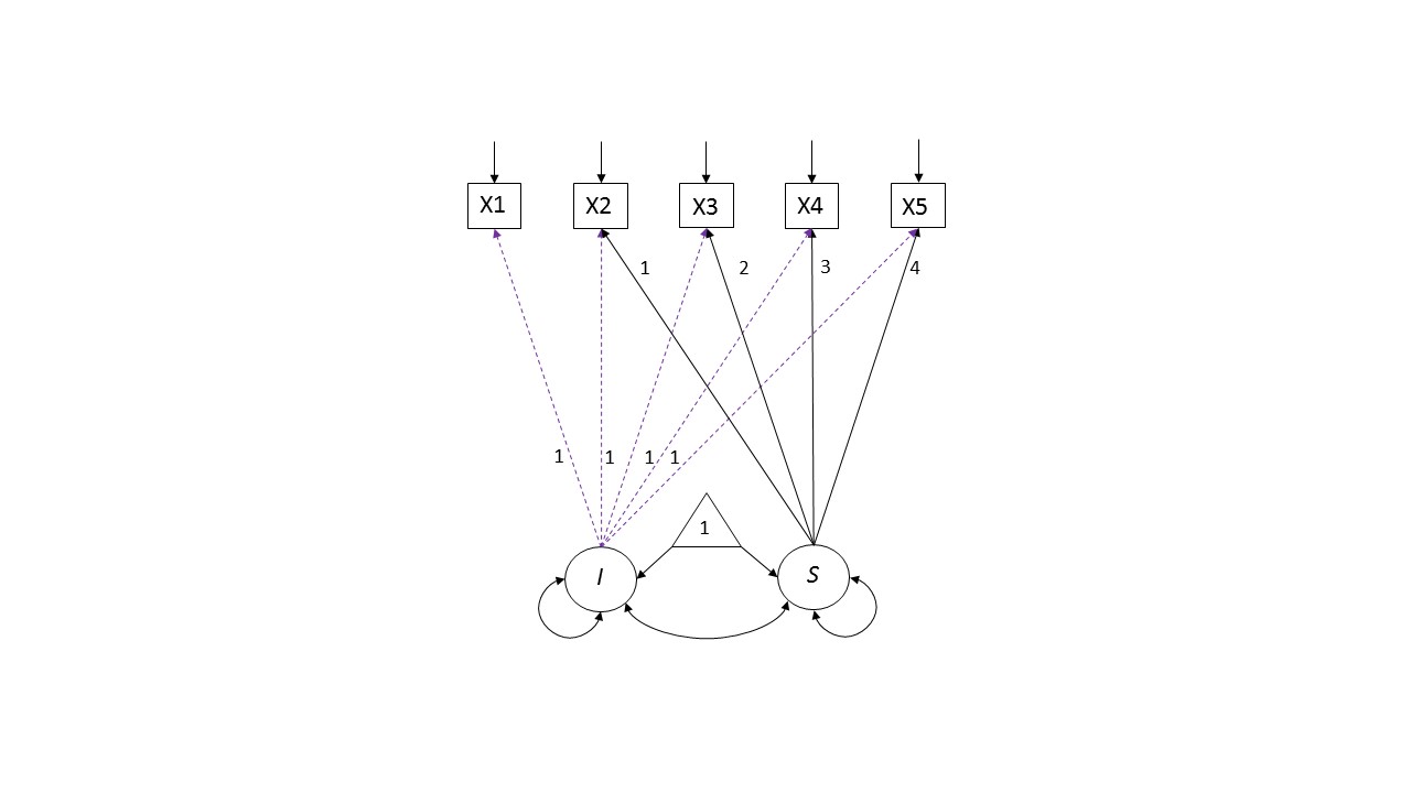
This pattern of weights allows us to represent the linear growth process assumed by our model:

x1 = i + 0s = i + e
x2 = i + 1s + e
x3 = i + 2s + e
x4 = i + 3s + e
x5 = i + 4s + e

Thus, if S = 0, then each x score is a function of the person's latent mean and an error term, e.

Here is the syntax for estimating the latent growth parameters in our simulated data. Notice that we are including a mean structure for this model because we want to estimate the means of our latent variables. And, in order to do so, it is best to fix the intercepts of the measured variables to 0. (Note: One can bypass these added parameters by using the growth() function in lavaan. This function knows what to do by default.)

	model <- '
	   # Latent Variable Definitions

		i =~ 1*x1 + 1*x2 + 1*x3 + 1*x4 + 1*x5
		s =~ 0*x1 + 1*x2 + 2*x3 + 3*x4 + 4*x5

	   # Regressions

	   # Misc
	   # Fix the intercepts of the measured variables
	   # to 0 and estimate the means of the 
	   # latent variables instead.

	     x1 ~0
	     x2 ~0
	     x3 ~0
	     x4 ~0
	     x5 ~0
	      i ~1
	      s ~1
	'

	results = sem(model, data=x)
	summary(results,standardized = TRUE, fit.measures=TRUE)

Recall that most of the parameters in this model are fixed. There are a few parameters that we are trying to estimate.

First, we want to know the mean of the latent intercepts. That is given in the section of the output called "Intercepts". In our example, the average intercept should be about 5, plus or minus some sampling error.

Second, we want to know the mean of the latent slopes. In our example, the average slope is about .1, plus or minus some error.

Third, we want to know the covariation between the intercepts and the slopes. In our simulation, we did not impose a correlation among these variables. In many real datasets, however, intercepts and slopes tend to covary negatively: People with low scores are more likely to increase over time than to decrease.

Finally, we want to know the variances of the estimated intercepts and slopes (see the output section titled "Variances." The significance tests for these parameters evaluate the whether there are significant individual differneces in these parameters. A common modeling strategy is to fix these variances to 0 and compare the fit of that model against one that allows them to be freely estimated. When the parameters are constrained to have a variance of zero, the intercepts (or slopes) are said to be fixed effects. When they are allowed to vary, the parameters are said to be random effects.

Putting it all together

Simulating Data from an SEM and Studying Parameter Recovery

Most of our errorts up to this point have focused on analyzing data using the framework of latent variable models. Part of the value of this framework is that it provides a way to analyze the implications of theoretical models. For example, using the tracing rules we described previously, we can see exactly what a model predicts about the associations among variables under different circumstances.

Another benefit of this approach is that we can generate data from these theoretical models. This is valuable because it allows us to examine whether a specific research design is capable of recovering the parameters of interest or testing the model in question.

Let us pull these themes together for a final example. Specifically, we will begin with a pair of simple theoretical models, determine the expected var-cov matrices implied by the models, simulate multiple datasets that adhere to that population var-cov structures, analyze the data in lavaan, and see how well it all works!

Generating the Population Var-Cov Matrix from a Model

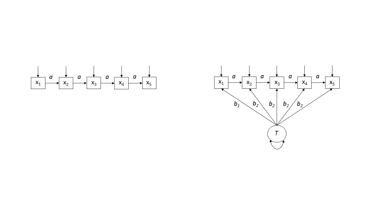
We will compare two developmental models of attachment stability. The first assumes that, over time, people's attachment styles change to some degree when their experiences are inconsistent with their expectations. Countering this change, however, is some degree of rigidity. Attachment styles tend to be self-perpetuating, for example. The left-hand panel of the figure below illustrates the core ideas in a path modeling framework. Each assessment of security (x1 - x5) is shaped by prior levels of security and sources of variance that are unrelated to previous states. This kind of model is sometimes referred to as an autoregressive longitudinal model.

If we assume a = .80, this implies the following var-cov matrix for all 5 measurement waves:

     x1   x2   x3   x4   x5
x1 1.00 0.80 0.64 0.51 0.41
x2 0.80 1.00 0.80 0.64 0.51
x3 0.64 0.80 1.00 0.80 0.64
x4 0.51 0.64 0.80 1.00 0.80
x5 0.41 0.51 0.64 0.80 1.00

We can derive this matrix using the tracing rules discussed previously. Here is some code that explicates the relevant paths in this example, placing each tracing in the proper place in a covariance matrix. In the examples we will discuss, we will assume unit variance; thus the covariane matrix is a correlation matrix.

	a = .8

	model1.cov = matrix(c(
		  1,   a, a^2, a^3, a^4,
		  a,   1,   a, a^2, a^3,
		a^2,   a,   1,   a, a^2,
		a^3, a^2,   a,   1,   a,
		a^4, a^3, a^2,   a,   1),
		5,5)
	rownames(model1.cov) = colnames(model1.cov) = c("x1","x2","x3","x4","x5")

	model1.cov

An alternative model is illustrated on the right-side of the figure. This model assumes that, in addition to the autoregressive processes described previously, there is a stable source of variance, T, contributing to measurements at each point in time. This model is a variant of a trait-state model.

Assuming that a = .30, and b1 = b2 = .50, the second model implies the following var-cov matrix for all 5 measurement waves:

     x1   x2   x3   x4   x5
x1 1.00 0.55 0.42 0.37 0.36
x2 0.55 1.00 0.62 0.51 0.48
x3 0.42 0.62 1.00 0.65 0.54
x4 0.37 0.51 0.65 1.00 0.65
x5 0.36 0.48 0.54 0.65 1.00

Here is some code that takes the path model/tracing derivations and creates the population covariance matrix with it. It is unbearable, but I've included it so I don't forget it later.

a = .3
b1 = .5
b2 = .5

model2.cov = matrix(1,5,5)

model2.cov[2,1] = model2.cov[1,2] = a   + b1*b2
model2.cov[3,1] = model2.cov[1,3] = a^2 + b1*b2 + b1*b2*a	
model2.cov[4,1] = model2.cov[1,4] = a^3 + b1*b2 + b1*b2*a + b1*b2*a^2	
model2.cov[5,1] = model2.cov[1,5] = a^4 + b1*b2 + b1*b2*a + b1*b2*a^2 + b1*b2*a^3

model2.cov[3,2] = model2.cov[2,3] = a   + b2^2 + b1*b2*a
model2.cov[4,2] = model2.cov[2,4] = a^2 + b2^2 + b1*b2*a + b2*b2*a + b1*b2*a^2	
model2.cov[5,2] = model2.cov[2,5] = a^3 + b2^2 + b1*b2*a + b2*b2*a^2 + b2*b2*a + b1*b2*a^3 + b1*b2*a^2	

model2.cov[4,3] = model2.cov[3,4] = a   + b2^2 + b2*b2*a + b1*b2*a^2
model2.cov[5,3] = model2.cov[3,5] = a^2 + b2^2 + b2*b2*a + b1*b2*a^2 + b2*b2*a + b2*b2*a^2 + b2*b1*a^3	

model2.cov[4,5] = model2.cov[5,4] = a + b2^2 + b2*b2*a + b2*b2*a^2 + b1*b2*a^3

rownames(model2.cov) = colnames(model2.cov) = c("x1","x2","x3","x4","x5")

model2.cov

Please note that verbally these two models make identical predictions in standard NHST Land: All correlations will be significantly different from zero. Also note that, if one of the correlation matrices shown above were to be observed in an emprical study, most researchers could use the data to advocate for either model. In psychology, we are not used to thinking about the structure of these associations. But the structure of the associations is what differentiates the two matrices. The power of latent variable modeling is that it allows us to appreciate this fact and provides us with tools to use it to our advantage.

Generating Random Normal Data from the Var-Cov Matrix

Now that we have derived the expected var-cov matrices under different theoretical assumptions, we can generate data based on those matrices for the purposes of simulations.

For this purpose, we will install and use a package called MASS. Once you've installed the package, you can load the library by using the library(MASS) command. You only need to use this once in a session.

The MASS library contains the mvrnorm() function--a function that generates multivariate normal data of any sample size based on a vector of means and the population variance-covariance matrix.

Let's generate two data sets using the two population covariance matrices we derived previously. We will use a sample size of 200 for each. And, because we are not concerned with the mean structure, we will set the population means for each variable to 0 (that is, we create a vector of five 0's).

	x1 = mvrnorm(n = 200, mu = rep(0,5), Sigma = model1.cov)
	x2 = mvrnorm(n = 200, mu = rep(0,5), Sigma = model2.cov)

Notice that if you compute the covariance matrix for these data sets, they'll be similar to, but not exactly equal to, the population matrices. The reason for the discrepancy is sampling error. Thus, each time we run the command, we generate data that are a bit different, even if they derive from the same model. The discrepancies will be more noticable with smaller sample sizes, of course.

Estimation in lavaan

Because we have two models, we'll build two different model statements and evaluate the models separately.

	model1 <- '
	   # Latent Variable Definitions
		
	   # Regressions
		x2 ~ a*x1
		x3 ~ a*x2
		x4 ~ a*x3
		x5 ~ a*x4

	   # Misc
	'

	results = sem(model1, data=x1)
	summary(results,standardized = TRUE, fit.measures=TRUE)

Notice that the estimate of the a parameter is close to the value we used to generate the population covariance matrix (a = .80). In other words, lavaan recovered the parameters well.

Let's try model2:

	model2 <- '
	   # Latent Variable Definitions
		T =~ NA*x1 + b2*x2 + b2*x3 + b2*x4 + b2*x5

	   # Regressions
		x2 ~ a*x1
		x3 ~ a*x2
		x4 ~ a*x3
		x5 ~ a*x4

	   # Misc
		T ~~ 1*T
	'

	results2 = sem(model2, data=x2)
	summary(results2,standardized = TRUE, fit.measures=TRUE)

Recall that the population values for this model were a = .30, b1 = b2 = .5. lavaan was able to recover these parameters accurately from the empirical data.

(As a useful exercise, try fitting both models to mismatched data.)

Now let's build a loop and compare the two models across multiple datasets generated from the trait-state population correlation matrix. We will evaluate the power to detect a difference in fit between the pure autoregressive model (model1) and the trait-state model (model2) using a chi-square difference test.

	trials = 1000
	p.values = rep(NA,trials)

	options(warn=2)
	for(i in 1:trials){
		
		flush.console()
		print(i)

		x2 = mvrnorm(n = 80, mu = rep(0,5), Sigma = model2.cov)
		x2 = data.frame(x2)
		results1 = try(sem(model1, data=x2))
		results2 = try(sem(model2, data=x2))

		# The p-value is stored as the second element of the 7th part
		p.values[i] = anova(results1,results2)[[7]][2]

	}

	sum(p.values < .05)/trials

Note: I added one additional trick here. Sometimes lavaan will not converge for various reasons. When the model failed to converge, the error 'breaks' the loop. This is awfully inconvienet for simulation work. The try() function tries to do something that has the potential to break. If it does produce an error, we get a message (options(warn=2)), but the loop keeps going. These errors merit close inspection, but I'm glossing over them for now.

This simulation will take a while to run; you may wish to use only 100 trials to see how this process works. We can see from these simulations that with a sample size of 80 we have relatively high power for detecting that one model performs better than the other via a change in chi-square test.

---

IPIP20 items 1 "I am the life of the party"," 2 "I don't talk a lot", 3 "I talk to a lot of different people at parties" 4 "I keep in the background"," 5 I sympathize with others' feelings", 6 "I am not interested in other people's problems", 7 "I feel others' emotions", 8 " I am not really interested in others", 9 "I like order", 10 "I get chores done right away", 11 "I often forget to put things back in their proper place", 12 "I make a mess of things", 13 "I have frequent mood swings", 14 "I get upset easily", 15 "I am relaxed most of the time", 16 "I seldom feel blue", 17 "I have a vivid imagination", 18 "I am not interested in abstract ideas", 19 "I have difficulty understanding abstract ideas", 20 "I do not have a good imagination",